Diffusing the mathematical equations of Diffusion Modelling

Over the past two years, the body of research on diffusion models has grown significantly. In this blog, I explain the foundations of diffusion models.

Denoising Diffusion probabilistic model has two steps in it:-

1. Forward Diffusion: Add gaussian noise at each step to the input
2. Reverse Diffusion: Approximate the denoised input at each step

Forward Diffusion

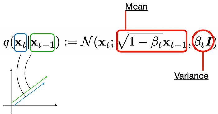
At every step we assume to generate noisy image conditioned on previous image using a normal distribution. This normal distribution, takes the image at previous step, rescales it by a factor of sqrt(1 — β_t) and adds tiny bit of noise with a variance of β_t. The schedule of β’s is defined such that β1<β2<β3<…<β_T, where T is the last step in forward iteration.

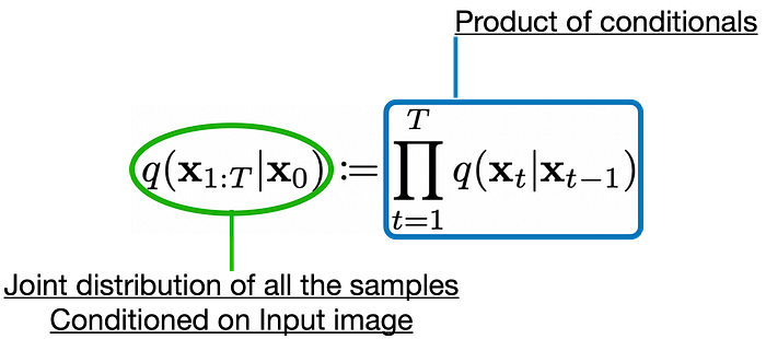
We can also define the joint distribution for all the samples that will be generated in this chain of forward diffusion starting from x1 till xT as

But since we are using such a simple distribution to generate samples in forward diffusion, cant we just jump to any t step in the forward chain using function composition? The answer is, Yes we can by using Normal distribution where mean is actual input rescaled by ⍺_t’s and variance is the corresponding noise added to it.

So, in case you want to sample images after t_steps of forward diffusion given input image, one can simply use the equation

Till now we have talked about conditional distribution of latent given the input q(xt | x0), but what happens to the marginal data distribution q(xt) as we move forward? Marginal distribution can be calculated using integration over the joint distribution of diffused data and actual input.